Formlagarna i härledning — Universums Historia

UNIVERSUMS HISTORIA | FORMLAGARNA I HÄRLEDNING | 2012VIII14 | a BellDHARMA production | Senast uppdaterade version: 2018-12-27 · Universums Historia

innehåll denna sida · webbSÖK äMNESORD på denna sida Ctrl+F · sök ämnesord överallt i SAKREGISTER · förteckning över alla webbsidor

HÄRLEDNINGARNA TILL FORMLAGARNA — Tabellen

FORMLAGARNAS HÄRLEDNING

TRIGONOMETRISKA | EXPONENTIELLA | LOGARITMISKA

Formlagarna, TextTabell med länkar till utförliga härledningar [SvEngelska — från originalförfattningarna i sammanställning från 1984]

Formlagarna — Textbaserad sammanställd tabell i PREFIXxSIN

Integralform				TANGENSFORM = derivata
dI/dx	=	Dn I	=	M	M; mo´dus (måttet); Derivatan = tangensformen; integranden
		I	=	∫ Mdx	Tangensformen för (derivatan till) I är M; Integralen för M är I
		I		M

DET ÄR OMÖJLIGT ATT FÅ EXAKT PIXELBASERAD ORIGINALÖVERENSSTÄMMELE VIA WEBBLÄSARE året 2012 — fullkomligt komplett OMÖJLIGT. Vad kan Programmakrna visa då PER precision? Visa. Ge ETT exempel.

— Det ser ut som att hela verksamheten går ut på just det: att INTE medverka till något PRECIST; att medvetet SÄNKA kvaliteterna. År efter år, Det enda som utvecklas är DE INTEGRERADE KOMPONENTERNA. Sänk skiten.

Formlagarna — Textbaserad sammanställd tabell med länkar till aktuella härledningar (i detta och övriga dokument)

Tabellen

	Integralform	TANGENSFORM
	integralen I	M derivatan y’
	Fundamentalintegraler	Elementära Derivator
	—————————	—————————
	funktion	derivata ¦ INTEGRAND
∫ I dx	I = ∫ M dx	M	Beteckning	Noteringar
trigonometriska:
cos	sin	– cos . . . . . . . . . . . . . . . .	TRIG1
–sin	cos	sin . . . . . . . . . . . . . . . .	TRIG2
n^–1cos nx	sin nx	– n(cos nx) . . . . . . . . . . .	TRIG3	Dn sin n(P) = –n(P)’cos n(P)
–n^–1sin nx	cos nx	n(sin nx) . . . . . . . . . . .	TRIG3	Dn cos n(P) = n(P)’ sin n(P)
–ln sinx	tan	1/sin² . . . . . . . . . . . . . .	TRIG4
ln cosx	cot	– 1/cos² . . . . . . . . . . . .	TRIG5
x asinx – √1–x²	asinx	– 1/√1–x² . . . . . . . . . . . .	TRIG6
x acosx + √1–x²	acosx	1/√1–x² . . . . . . . . . . . .	TRIG7
x atanx – ln√1+x²	atanx	1/(1+x²) . . . . . . . . . . . .	TRIG8
x acotx + ln√1+x²	acotx	– 1/(1+x²) . . . . . . . . . . . .	TRIG9	acot x = atan (1/x)
exponentiella:
—	(P)^a	a(P)^a^–1Dn(P) . . . . . . . . .	EXP7	exponentialDerivatan
x^a⁺¹(a+1)^–1	x^a	ax^a^–1 . . . . . . . . . . . . . . . .	EXP8	exponentialIntegralen, a≠–1 i ∫ I dx
—	(P)ⁿ⁺¹/(n+1)	(P)ⁿDn(P) . . . . . . . . . . .	EXP7	exponentialIntegralen, n≠–1
—	(x^a⁺¹)/(a+1)	x^a . . . . . . . . . . . . . . . . . .	EXP7
Se partialintegralen	AB	A(DnB) + B(DnA) . . . .	EXP5	produktDerivatan
—	A/B	[B(Dn A) – A(Dn B)]/B²	EXP6	kvotDerivatan
logaritmiska:
—	e^(P)	e^(P)Dn(P) . . . . . . . . . . . .	LOG2	exponentDerivatan
e^zx/z	e^zx	ze^zx . . . . . . . . . . . . . . . . . .	LOG2
e^x	e^x	e^x . . . . . . . . . . . . . . . . . .	LOG1
—	B^(P)	B^(P)Dn(P)lnB . . . . . . . . .		se nedan [1]
B^x(lnB)^–1	B^x	B^xlnB . . . . . . . . . . . . . . . .		samma som e^zx, B=e^z
—	ln(P)	Dn(P)/(P) . . . . . . . . . . . .	LOG5	logaritmDerivatan
x(ln x – 1)	ln x	1/x . . . . . . . . . . . . . . . . . .	LOG6	logaritmDerivatan, logaritmIntegralen

[1] ............................. B=e^a; a=lnB; Dn e^a(P) = e^a^(P)[ Dn(aP) = aDn(P) ] = B^(P) lnB·Dn(P); [ln e = 1]

Potensderivatan

Sammanställning — kungsderivatorna från logaritmderivatan

[(P)^Q]’ = (P)^Q[Q(P)’/(P) + Q’ln(P)] .......................... Allmänna PotensDerivatan

Q=konstant=n [(P)ⁿ]’ = (P)ⁿ[Q (P)’/(P)] = n(P)ⁿ^–1Dn(P) ................ ExponentialDerivatan (variabeln i Basen);

P=konstant=e [e^Q]’ = e^QQ’ln(e)] = e^QDn(Q) ................................. ExponentDerivatan (variabeln i Exponenten)

P och Q, Vilka Som Helst Uttryck, Konstanter Eller Funktioner.

Dn synkoperar »derivatan-tangensformen (till, för, av …)»

Formlagarna

FORMLAGARNA — från M2001_3.wps

The Form Laws

DESCRIBING — descriptive — WORDS ARE MISSING IN MODERN ACADEMY

MATHEMATICS IN GENERAL and physics in particular can NOT be described, explained or related with the available terms, concepts and statements in the modern academic teaching system. The presentation in UniversumsHistoria RELATES the math-basics from NOLLFORMSALGEBRAN in ATOMTRIANGELN. In parallel with the presentation in general, the different aspects are related, exemplified and discussed wherever possible. The specific equational parts are listed in The List with detailed references (actual links to quotes, descriptions, examples and comparisons) for further inspection. The List includes Physics.

På den svenska översättningsportalen http;//tyda.se/ finns ingenting liknande »räknelagar» på engelska;

— Termen eller begreppet LAG existerar över huvud taget inte i den moderna akademins MATEMATISKA vokabulär:

— Jämför MAC-citatet med MATEMATIKENS 5 GRUNDLAGAR — vi upptäcker lagar, vi kan härleda dem; de framträder ur en helt enkel mönstergrund. Men den finns inte upptagen, ens noterad eller omnämnd, i modern akademi.

— SÅ: HUR beskriver man ÄMNET?

Man får IMPROVISERA — med ände i att speciellt modernt akademiskt meriterade A-studenter som LÄSER ALLT VAD MÄNNISKOR SKRIVER SOM OM DE SJÄLVA STODE HÖGST UPP PÅ INTELLIGENSSTEGEN missar målet i framställningen — vilket SOM VI VET resulterar i att A-studenten ANSER sig vara uppkopplad mot en TOK, tills plötsligt hela draperiet dras undan och sanningen uppdagas:

— Matematikens RELATERADE domäner KAN INTE BESKRIVAS MED HJÄLP AV DEN MODERNA AKADEMINS vokabulär EFTERSOM den TYPEN redan från början (under 1800-talet) utformades i tanken om att MÄNNISKAN HAR SKAPAT MATEMATIKEN (MAC-citatet): MAC uppfinner, inte härleder.

Här tillämpas INTE den fasonen: A-studenterna i modern akademi har ingenting att hämta här. Helt rent.

— RÄKNELAGAR kan då på engelska bli något så töntigt som »RECKONING LAWS» — för att referera de BESKRIVBART härledande grunderna.

Formlagarna i utförliga härledningar [SvEngelska]

Med fortsättning från NOLLFORMSALGEBRAN

Form laws

Form laws · derivative, differential and integral calculus from The Position Form [POSITIONSFORMEN]

Positionsformen

^{______________________________________________________}

Dn y = y’ = dy/dx = (y₀–y)/(x₀–x) = (y₀–y)/dx — the position form — differentialkvoten [»Differential Quotient»]

^{______________________________________________________}

Developing and Deducing The Form Laws

Instead of using the position form for each case when we need to find a specific derivative, it is both much more convenient and effective to find the derivatives to the elementary mathematical functions once and for all, write them up in a table [FORMLAGARNA] and then use these more general achieved results in all kinds of problems. The following workout shows the general derivatives of the three elementary functional blocks named exponential (EXP), trigonometric (TRIG) and logarithmic (LOG) as follows. These are referred to by and connected with the corresponding hyperlinks in The General Table.

General deriving method

The following derivations will use any of the simplest and most direct available connections in the above given rank of the equivalents here named the position form. For each form law, the appropriate connection is written out — clarifying how the deduction has been made. If nothing else is mentioned, the term y will be used for the functional result, the term x for the functional variable and the term C for any arbitrary numeric constant. As far as possible, the integrals corresponding to the derivatives will be given directly along with each form-law.

In general, the term (P) will also be used to represent any arbitrary composition of functions in x — as explicitly denoted, starting from EXP(7).

— The abbreviation »Dn» is used here as a more clarifying term before the more conventional »D» for derivative of or derivative to — as also, in general in calculus in this presentation, the capital D and others are generally utilized for general algebraic coefficient purposes.

Exponentiella

Exponential functions

Coefficients in Derivatives

1. Dn Cy = C (Dn y)
∫ Cy’ = C ∫ y’
Dn Cy = d(Cy)/dx = C(dy/dx) = C(Dn y)

Single variable Derivative

2. Dn x = 1
∫ 1dx = x
y = x , y₀ = x₀
Dn x = (x₀–x)/(x₀–x) = 1

Constant Derivative — se utförligt i NOLLINTEGRALEN

3. Dn C = 0
∫dC = ∫ 0 = 0
y = y₀ = C
Dn C = dC/dx = 0 = (y₀–y)/dx = (C–C)/dx = (0)/dx = 0 ;
dy/dx = 0/dx=0 ; dy=0dx ; ∫ dy = ∫ 0 dx = 0 ∫ dx = 0·x = 0

Comment:

Note that derivatives to constants have no relevant meaning IN RELATED MATHEMATICS [NOLLFORMSALGEBRAN]: constants have no variation. Analytically IN RELATED MATHEMATICS — hence — a derivative to a constant does not exist. By the same reason constants have no integral representation — as here clearly derived. Note that this definition cannot be reached in MAC because of the modern idea defining »Δx=dx»; RELATED mathematics can not be explained on such a basis.

— See exemplified thorough description in NOLLINTEGRALEN where the modern standard is cited and compared.

Sum Derivatives

4. Dn (x₁+ x₂+ x₃+ … + x_n) = Dn(x₁) + Dn(x₂) + Dn(x₃) + …+ Dn(x_n)
∫ (x₁+ x₂+ x₃+ …+ x_n)dx
= ∫x₁dx + ∫x₂dx + ∫x₃dx + …+ ∫x_ndx
Dn (x₁+ x₂+ x₃+ … + x_n) = d(x₁+ x₂+ x₃+ … + x_n)/dx =
= d(x₁)/dx + d(x₂)/dx + d(x₃)/dx + …+ d(x_n)/dx

Product Derivative

5.          Dn AB = A(Dn B) + B(Dn A)
Derivative to Product from two x-dependent factors
y_A = A;   y₀ = y+dy = A+dA
y_B = B;   y₀ = y+dy = B+dB
y            = AB
y₀           = (y+dy)_A(y+dy)_B
             = (A+dA)(B+dB)
             = AB+AdB + BdA+dAdB
y₀ – y     = AB+AdB + BdA+dAdB – AB
             = AdB + BdA+dAdB
             = AdB + dA(B+dB)_Û_B
             = AdB + BdA ;
d(AB)/dx           = (y₀–y)/dx = (AdB + BdA)/dx
             = (AdB/dx) + (BdA/dx)
             = A(dB/dx) + B(dA/dx)
             = A(Dn B) + B(Dn A)
Dn AB = A(Dn B) + B(Dn A)
(AB)’    = A · B’     + A’ · B

Comment:

PARTIAL INTEGRALS — Se utförligt i PARTIELL INEGRATION

The product derivative is a highly versatile instrument all categories in calculus. Besides an excellent tool in verifying integral results, its »reversal» contains the specially powerful method for integrals in partial integration. Through the differential equation

d(AB) = AdB + BdA giving

AdB = d(AB) – BdA

we observe that

AdB = AB’dx , d(AB) = (AB)’dx , BdA = BA’dx , giving

The Partial Integral

∫ AdB = AB – ∫ BdA

The partial integral, featuring an integral equation, can be applied in two distinct methodical parts, METHOD 1 and METHOD 2:

METHOD 1 — Without equivalent :

∫ AdB = AB – ∫ BdA

A given integral form is conceived as the

one part (left) of the rank in the Partial:

∫ AdB = AB – ∫ BdA ........................ partial integral, Method 1

METHOD 2 — With equivalent :

∫ AdB = AB — ∫∫ dB dA

A given derivative integral (Þ) is conceived

as one of the Partial’s factors:

∫ AdB = AB – ∫ BdA ........................ partial integral, Method 2

To (highly) simplify the handling of the partial integral we will in this production use the general partial chart

∫ f (x) d[·] = f (x)[·] – ∫ [·]d[f (x)] ........................ Method 1

∫ [·] f (x) dx = [·] ò f (x) dx – ∫∫ f (x) dx d[·] ......... Method 2

[·] the unknown, denotes an arbitrary input-function

[not necessarily, but generally of the type x]

Se utförligt med exempel i PARTIELL INEGRATION

In general problems of integral calculus, it is more by rule than exception to find use for either of these two powerful integral methods.

— Both methods are explained in detail by simple examples in the section PARTIELL INEGRATION.

Quotient Derivative

6.          Dn A/B = [B(Dn A) – A(Dn B)]/B²
Derivative to Quotient between two x-dependent factors
y_A = A;   y_0A = y_A+dy = A+dA
y_B = B;   y_0B = y_B+dy = B+dB
y            = A/B
y₀ – y     = (y+dy)_A/(y+dy)_B – A/B
             = (A+dA)/(B+dB) – A/B
             = [B(A+dA) – A(B+dB)]/B(B+dB)
             = [BA+BdA – AB – AdB]/B(B+dB)
             = [BdA – AdB]/B(B+dB)_Û_B
             = [BdA–AdB]/B² ;
d(AB)/dx           = (y₀–y)/dx = (1/dx)[BdA – AdB]/B²
             = [B(dA/dx) – A(dB/dx)]/B²
             = [B(Dn A) – A(Dn B)]/B²
Dn A/B             = [B(Dn A) – A(Dn B)]/B²

Exponential Derivative

7. Dn (P)^a = a(P)^a^–¹Dn(P)
a–1=m ; Dn (P)^m⁺¹ = d(P)^m⁺¹/dx = (m+1)(P)^mDn(P) ;

Exponential Integral
∫(P)^mDn(P)dx = (P)^m⁺¹/(m+1) ; m ≠–1
(P) = (Ax^k + Bx^l + Cx^m +…)
y = (Ax^k + Bx^l + Cx^m +…)^a = (P)^a
y = (P)^a , y₀ = (P)₀^a
(P) = X
y = X^a , y₀ = X₀^a
dy/dx = [X₀^a – X^a]/dx = [[X + dX]^a – X^a]/dx
(X+dX)^a inserted for (a+b)ⁿ in the binomial theorem:
X^a + X^aa(dX/X) + X^aa(a–1)(dX/X)²/2! + X^aa(a–1)(a–2)(dX/X)³/3!
+ X^aa(a–1)(a–2)(a–3)(dX/X)⁴/4! + … + (dX)^a
Subtracting X^a and then dividing by dx, only one term can eliminate dx, the second in the rank above, the X^aa(dX/X). The remaining is hence :
dy/dx X^aa(dX/dxX) = aX^a^–1 dX/dx = aX^a^–1 Dn X dx/dx = aX^a^–1 Dn X ;
Dn (P)^a = a(P)^a^–1 Dn (P)

NOTE on transition from positions (dx) to values (Δx) — see also in DERIVATA OCH INTEGRAL, dx 0:

— In MAC there is no distinction between Δx (IN RELATED MATHEMATICS a difference) and dx (IN RELATED MATHEMATICS a differential=position=point) — se quote »Δx=dx» — meaning »general chaos» in MAC in defining calculus basics: not one person on Planet Earth understands — can EXPLAIN to others — modern academy calculus; guaranteed.

— In RELATED MATHEMATICS this »difficulty» is eliminated by observing the natural properties of positions (differentials as part of zero=point=nothing) and values (intervals=differences to zero). See detailed definitions and descriptions in NOLLFORMSALGEBRAN, explicitly in MÄSTARLOGIKENS HUVUDSATS: there are no limitless quantities: points (0) does not add to intervals.

Exponential Derivative, simple case of (7) with (P)=x

8. Dn x^a = ax^a^–¹

Exponential Integral

∫ x^m dx = x^m⁺¹/(m+1) ; m ¹ –1

Trigonometriska

Trigonometric functions in PREFIXxSIN

We use the Series for sine and cosine [Sinus&CosinusSERIERmed i] [Sinus&CosinusSERIERutan i], a in radians.

sin a = 1 – a²/2! + a⁴/4! – a⁶/6! + a⁸/8! – a¹⁰/10! + …

cos a = a – a³/3! + a⁵/5! – a⁷/7! + a⁹/9! – a¹¹/11! + …

Sine Derivative

1. Dn sin = –cos

∫ –cosx dx = sin x ; ∫ cosx dx = –sin x
Derivation term by term via form law EXP4&EXP8 in sine series gives –cos:
0 – 2a/2! + 4a³/4! – 6a⁵/6! + 8a⁷/8! – 10a⁹/10! + … ;
– a + a³/3! – a⁵/5! + a⁷/7! – a⁹/9! + …

Cosine Derivative

2. Dn cos = sin

∫ sinx dx = cos x
Derivation term by term via form law (EXP4&EXP8) in cosine series gives sine:
1 – 3a²/3! + 5a⁴/5! – 7a⁶/7! + 9a⁸/9! – 11a⁹/11! + …
1 – a²/2! + a⁴/4! – a⁶/6! + a⁸/8! – a⁹/10! + …

Angle Coefficient Derivatives, Sine and Cosine

3. Dn sin na = – n(cos na)

∫–n(cos nx) dx = sin nx ; n∫(cos nx) dx = –sin nx

Dn cos na = n(sin na)

             ∫ n(sin nx) dx = cos nx
By example from the sine series, we study how a multiple n of the angle a duplicates out to a constant coefficient on derivation (The cosine derivation then extracts directly by mind) we use EXP4&EXP8;
sin na                = 1 – n²a²/2! + n⁴a⁴/4! – n⁶a⁶/6! + n⁸a⁸/8! – …
Dn sinna           = 0 – n²a + n⁴a³/3! – n⁶a⁵/5! + n⁸a⁷/7! – …
Dn sinna           = –    [n²a – n⁴a³/3! + n⁶a⁵/5! – n⁸a⁷/7! + …
                          = –n[na – n³a³/3! + n⁵a⁵/5! – n⁷a⁷/7! + …
                          = –n[cos na]
MORE GENERALLY if a is any composite function of x as (P) it holds that
Dn sin n(P) = – n Dn(P) cos n(P)
Dn cos n(P) =    n Dn(P) sin n(P)
exemplified in development through
sin n(P)             = 1 – n²(P)²/2! + n⁴(P)⁴/4! – n⁶(P)⁶/6! + n⁸(P)⁸/8! – …
Dn sinn(P)        = 0 – n²(P)Dn(P) + n⁴(P)³Dn(P)/3! – n⁶(P)⁵Dn(P)/5! + n⁸(P)⁷Dn(P)/7! – …
Dn sinn(P)        = –    [n²(P)Dn(P) – n⁴(P)³Dn(P)/3! + n⁶(P)⁵Dn(P)/5! – n⁸(P)⁷Dn(P)/7! + …
                          = –nDn(P)[n(P) – n³(P)³/3! + n⁵(P)⁵/5! – n⁷(P)⁷/7! + …
                          = –nDn(P)[cos n(P)]

In the article THE TANGENT FORMS IN TRIGONOMETRY the derivatives for tangent and cotangent have already been derived (a summation is given below). We will however rejoin through an alternative way in using the earlier derived form law EXP6 to show a derivation more consistent (and easier) with this section presentation.

Developing the sine function (II)

4. Dn tan = 1/sin²

∫ 1/(sinx)² dx = tan x
We apply EXP6 ; Dn A/B = [B(Dn A) – A(Dn B)]/B²,
tan = cos/sin ;
Dn tan = Dn cos/sin = [sin Dncos – cos Dnsin]/sin²

= [sin² + cos²]/sin² = 1/sin²
Adding the angle coefficient n to x, we can follow the derivation above using TRIG3 and see that the result becomes
Dn tan nx = n/(sin nx)²

5. Dn cot = Dn 1/tan = –1/cos²

∫–1/(cosx)² dx = 1/tanx
We apply EXP6 ; Dn A/B = [B(Dn A) – A(Dn B)]/B²,
Dn 1/tan = Dn sin/cos = [cosDnsin – sinDncos]/cos²

= [–cos² –sin²]/cos² = –1/cos²
Adding the angle coefficient n to x, we can follow the derivation above using TRIG3 and see that the result becomes
Dn cot nx = –n/(cos nx)²

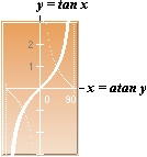
Arkusfunktionernas Tangensformer

Arc functions Tangent forms

These derivations appear illustrated in THE TANGENT FORMS IN TRIGONOMETRY. We will here give a corresponding short strict formal survey of these mentioned more detailed derivations.

By relating the angle-zero index for the tangent forms sinx, –cosx, –sinx, and cosx to negative y-axis, respectively 1/–sinx, 1/cosx, 1/sinx and 1/–cosx, and additionally express all x as Arc sine [asin] and Arc cosine [acos] according to respectively asiny, acosy, asiny and acosy, and then finally rotate the coordinate system positively by an exact quarter of a turn along with shifting the terms xy respectively accordingly as asin–x, acosx, asinx and acos–x, the expressions are directly obtained for the arc tangent functions as [Dn asin–x = 1/√1–x²], [Dn acosx = 1/√1–x²], [Dn asinx = –1/√1–x²] and [Dn acos–x = –1/√1–x²].

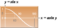
6. Dn asin x = –1/√1–x² ;
y = asin x ; Dn y = –1/siny = –1/√1–[cos y]²

∫–(1/√1–x²) dx = asin x
With an angular coefficient n
[See also The derivatives with angle coefficient] we find
Dn asin nx = –n/√1–(nx)²

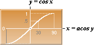
7. Dn acos x = 1/√1–x² ;
y = acos x ; Dn y = 1/cosy = –1/√1–[sin y]²

∫(1/√1–x²) dx = acos x
With an angular coefficient n
[See also The derivatives with angle coefficient] we find
Dn acos nx = n/√1–(nx)²

Adopting the same method as in (6) and (7) above, the tangent forms for atan and acotan are obtained as

8. Dn atan x = 1/1+x² ;
= 1/[1+(tan y)²

∫(1+x²)^–1 dx = atan x
With an angular coefficient n
[See also The derivatives with angle coefficient] we find
Dn atan nx = n/1+(nx)²

9. Dn acot x = –1/1+x² ;
= –1/[1+ (cot y)²]

∫–(1+x²)^–1 dx = acot x = atan (1/x)
With an angular coefficient n
[See also The derivatives with angle coefficient] we find
Dn acot nx = –n/1+(nx)²

Logaritmiska

Logarithmic functions

See INTRODUCTION with the Deduction of The Natural Logarithm

Logarithmic functions

Continuing on Logarithmic functions

REGULAR DERIVATIONS logarithmic functions

Exponent Derivative, simple case

1. Dn e^x = e^x

Exponent Integral:
∫ e^x dx = e^x.
From the Deduction of The Natural Logarithm we have the exponent of the natural logarithm as
(1+1/∞)^∞x = (1+x/∞)^∞= e^x
= 1 + x + x²/2! + x³/3! + x⁴/4! + x⁵/5! + … + x^m/m!
Derivation term by term through EXP4&EXP8 gives
Dn e^x = 0 + 1 + 2x/2! + 3x²/3! + 4x³/4! + 5x⁴/5! + …+ mx^m–¹/(m–1)!
Dn e^x = 1 + x + x²/2! + x³/3! + x⁴/4! + …+ x^m–¹/(m–1)! = e^x
As we see, the result is just pushed net intact!

Exponent Derivative, natural logarithm

2. Dn e^(P) = e^(P)·Dn(P)

Exponent Integral, general (i.e., regular):
∫ e^(P)·Dn(P) dx = e^(P).
Superseding x by (P) in the ranks of LOG1 above gives
e^(P) = 1 + (P) + (P)²/2! + (P)³/3! + (P)⁴/4! + (P)⁵/5! + …+ (P)^m/m!
Derivation through EXP4&EXP8 gives
Dn e^(P) = 0 + Dn(P) + 2(P)Dn(P)/2! + 3(P)²Dn(P)/3! + …+ m(P)^m^–1Dn(P)/m!
Dn e^(P) = Dn(P)[1 + (P) + (P)²/2! + (P)³/3! + (P)⁴/4! + …+ (P)^m/m!]
The part within square brackets has the form e^(P), hence Dn e^(P) = Dn(P)·e^(P)
As a numeric constant can be moved freely between the parts of a rank [see EXP1] we receive for the special case where Dn(P)=m=constant
Dn e^(P)Dn(P)^–1 = e^(P) ,
∫ e^(P) dx = e^(P)Dn(P)^–1 ; i.e.,
∫ e^mx dx = e^mx/m

Exponent Derivative, general logarithm — se HÄRLEDNINGEN TILL e

3. Dn B^x = B^xlnB
∫ B^xlnB dx = B^x
B = e^m ; m = lnB ; B^x = e^mx
Dn B^x = Dn e^mx = [e^mx·Dn mx], See LOG2, = e^mx·m
Dn B^x = e^mxm = B^xlnB

^{_ _ _ _ _ _ _ _ _ _ _ _ _ _ _ _ _ _ _ _ _ _ _ _ _ _ _ _ _ _ _ _ _ _ _ _
_ _ _ _ _ _ _ _ _ _ _ _ _ _ _ _ _ _ _ _ _}

LOGARITHM FUNCTION’s x-CONSTANT

a = (lnB)^–¹

From Proof of (1+1/∞)^∞=e in Deduction of The Natural Logarithm we remind the tangent form to the logarithm function as

k = y/a = B^x/a, with a as the constant on the x-axis ;

Through the form law in (3) above we then receive

k = Dn B^x = B^xlnB

1/a = lnB ;

a = 1/lnB

^{_ _ _ _ _ _ _ _ _ _ _ _ _ _ _ _ _ _ _ _ _ _ _ _ _ _ _ _ _ _ _ _ _ _ _ _
_ _ _ _ _ _ _ _ _ _ _ _ _ _ _ _ _ _ _ _ _}

Fixing the details

As earlier related in MATHEMATICS FROM THE BEGINNING chapter one (see The Reckoning Laws, The basic logarithm laws) we have through the connections

B^x=P, x = ^BlogP (here simplified as BlogP) that B^BlogP = P

Correspondingly we have through

e^x = (P), x = ln P, that e^ln^(P) = (P)

With this result we supersede the exponent to e in our recently derived exponent derivative LOG2,

Dn e^(P) = e^(P)·Dn(P), by ln(P) giving

Dn e^ln^(P) = e^ln^(P) Dn ln(P)

As the equivalent to e^ln^(P) is (P) we use this equality in the right part rank above which then gives us the form law

4. Dn (P) = (P)·Dn ln(P) = d(P)/dx = (P)d[ln(P)]/dx
Expressed in Dn ln(P), this LOG(4) gives us the highly context central logarithmic form law

Logarithm Derivative

5.          Dn ln(P) = Dn(P)/(P)
We observe that in introducing a constant factor C to the (P)-function as (PC) we receive exactly the same result
Dn ln(PC) = Dn(PC)/(PC) = C · Dn(P)/(PC) = Dn(P)/(P)
That is: constant factors are completely ignored by logarithm derivatives;
|             Special application; R = √(x²+a) ; (P) = x+R ;
|             Dn R, see EXP7, = Dn(x²+a)^1/2 = (1/2)(x²+a)^–1/22x = xR^–1 ;
|             Dn ln(x+R) = (P)’/(P) = (1+xR^–1)/(x+R) = R^–1(R+x)/(x+R) = R^–1 .
|             ∫ R^–1dx = Dn ln(x+R) , R = √(x²±a)
Continue
Dn(P)/(P) = [d(P)/dx]/(P) ; Dn ln(P) dx = d(P)/(P) ;

Logarithm Integral, (special)
∫ d(P)/(P) = ∫ Dn ln(P) dx = ∫ d[ln(P)] = ln(P)
Applying the constant-independency character above with C as constant yields the highly original even more general logarithm integral
∫ d(P)/(P) = ∫ d[ln(P)] = ln(PC)
whereas Dn ln(PC) = (PC)’/(PC) = (P)’/(P).
i.e., the logarithm integral solution generates an admittance of conditions not explicitly included in the integrand (the default is 1 in the solution).

NOTE. The more truly regular term Logarithm Integral is found by the following development [The integral to LOG5 as ”logarithmic” more appeals to the general group in the form laws we are studying than the actual expression; compare the following].

Advanced exercise (writing mixed Dn(P) and (P)’):
In applying the Product Derivative EXP5 on LOG5 through the function
(P)’ln(P) we receive
(P)’ln(P) = [(P)ln(P)]’ = (P) · Dn ln(P) + Dn (P) · ln(P) ;
= Dn(P) + Dn (P) · ln(P) ;
(P)’ln(P) – Dn(P) = (P)’ln(P) ;
Dn[(P)ln(P) – (P)] = Dn(P) · ln(P) ; Hence

Tangent-Logarithm Integral, advanced (regular)
∫ Dn(P) · ln(P) dx = (P) · ln(P) – (P)

Especially for (P)=x we receive the simple-case

6. Dn ln x = 1/x
d(ln x)/dx = 1/x ; d(ln x) = dx/x ;
∫ dx/x = ∫ d(ln x) = ln x

On behalf of the entirety we must here and via LOG5 note the similarity with the exponential form law EXP7. As the latter is

Dn(P)^a = a(P)^a^–¹Dn(P) = a(P)^aDn(P)/(P)

we receive from this rank out of its first and last parts, and thereby the equality with LOG5,

7. Dn(P)^a/a(P)^a = Dn(P)/(P) = Dn ln(P)

Hence with the middle link common to the both functional classes exponential and logarithmic functions. With these details we have made the arrangements and can return to physics in the main context.

Of the form laws above, as recently noted, the ranks around LOG5 are of vital and immense significance to (the functional forms within) physics. If we plainly formally incept a departure from a mathematical expression of the form

(8) e ^f^(t) = (P) = (a±F)

f (t) time function (= C t), C an arbitrary (optimal) proportionality coefficient

t actual time

a top or limiting value (”my roof” to the physical quantity)

F actual corresponding functional momentary value with t as the functional variable

we receive

(9) f (t) = ln (P) = ln (a±F)

If we now apply (9) for ln(P) into (4) [= Dn(P) = (P) · Dn ln(P) ] we receive through the equality Dn ln(P) = Dn f (t) number (4) on the form

(10) Dn (P) = (P) · Dn f (t) ....................... (P)C

In this equality Dn f (t), with f (t) = C t from (8), gives us Dn C t = C [see EXP1&EXP2], that is Dn f (t)=C. Hence

Dn(P) = (P)C from no(10). For Dn(P) = Dn(a±F) from no(8) we obtain by the same application of the sum derivative EXP4 that

Dn (a±F) = Dn a ± Dn F

As earlier, a is a constant which from no(8) gives in total

Dn (a±F) = 0 ± Dn F = Dn(P), = ±dF/dt.

Important

As we see of this, which is important to observe although seemingly tiny in its own existence, the polarity of the quotient dF/dt follows from the polarity of F as dF/dt just in another expression of the F-derivative. In explicit terms we hence must observe that

± Dn F = dF/(±dt)

In other words: the time factor receives the polarity of F. To simplify the proceeding derivations we now, with this decisive condition in mind, can ignore the explicit inclusion of the ±-sign in our expressions and then later on resume by giving the more exact formula. We hence have

Dn (a+F) = Dn F = Dn(P), = dF/dt.

Compiling all this together we have, in other words,

(11) Dn(P) = (P)C

= Dn F ...............

= dF/dt ................ dF/dt = F’ ; dF/F’ = dt

= (a+F)C

= (P) · Dn ln(P)

As we see, the equivalents marked above at the rightmost is absolutely identical to the differential quotient [The Position Form] outlined and discussed from the beginning of this workout; No mess.

From these central ranks, number 3 and 4 from top of (11), we now receive the derivative equation or the variant [VARIANT]

(12) dF/dt = (a+F)C [ = (a+F)’ = (P)’ = (P) f ’(t) = F’ ]_{JUST SUMMING}

................................................................ take some time to check that things fit

with the differential equation

dF/(a+F) = C dt

That’s it.

The only thing that remains now — when we have mounted the whole building and got all the furniture and the computers in at all their proper places and the kitchen filled with good bread and fresh tomatoes and lots of good tea — is to paint the house with energy. That is, to apply an integral to the whole construction.

The solution to the differential equation

PREPARING FOR PRACTICAL PHYSICS

Object: dF/(a+F) = C dt

AS WE SEE from all integrands of the type dF/(a+F) with the differential equation

dF/(a+F) = Kdt

there is via the logarithm derivative LOG5, Dn ln(P) = Dn(P)/(P), given the corresponding (separate) integrals, each for each side of the rank, as

_F _t

(13) ∫ dF/(a+F) = ∫ Kdt ;

⁰ ⁰

We observe for exact clarity that Dn(a+F)=Dn(F), meaning the same as d(a+F)=d(F) so that the principal Logarithm Integral from LOG5,

∫ d(P)/(P)=ln(P), still holds independent of whether a separate additive constant is present or not in the integrand’s denominator. The general interpretation of the integral terminology here used is explained in INSÄTTNINGSGRÄNSER.

_F _F

∫ dF/(a+F) = [ ln(a+F) ] = ln(a+F) – ln(a+0) =

⁰ ⁰

= ln(a+F) – ln(a)

Recall the logarithm laws;

= ln (a+F)/a = Kt

The solutions by the exponent expressions in total then become

ae^Kt = a+F

ae^Kt – a = F ;

(14) F = a(e^Kt – 1)

If the integration in the F-integral instead is taken between F and any arbitrary starting value b, [we then use the constant-independency quality in LOG5,

Dn ln(PC) = Dn(PC)/(PC) = Dn(P)/(P) ]

(15) ∫ dF/(a+F) = ln(a+F) – ln(a+b) = Kt =

= ln[(a+F)/(a+b)]

the solution in fundamental integrals in total for this more general case becomes

e^Kt = (a+F)/(a+b)

(a+b)e^Kt = a+F

(a+b)e^Kt – a = F = ae^Kt + be^Kt – a
= ae^Kt – a + be^Kt = a(e^Kt – 1) + be^Kt ;

(16) F = a(e^Kt – 1) + be^Kt

We observe that as the b-factor belongs to the F-factor then also the polarity of b follows from the polarity of F as well as also the polarity of t follows from the polarity of F, as earlier explicitly explained (see Important). That is, the F-polarity determines the two other actual factor-poles bt.

This more general case with an offset factor b then corresponds to exactly the same differential equation as without the b-factor according to the observed constant-independency property of LOG5. That is,

ln[(a+F)/(a+b)] ”=” ln[(a+F)],

See Note below

as both these give the same derivative

——— = Dn ln[(a+F)/(a+b)] = Dn ln[(a+F)]

a+F

For the b-factor [the entire (a+b)-parenthesis] that is:

its condition cannot be formulated or expressed in the integrand

without changing the entire status of the expression itself.

NOTE:

We observe the trap: the two expressions on each side of the marked ”=” cannot compile directly as equal as this (in general) would give us the obscure result

(a+F)/(a+b) = (a+F) ; 1 = (a+b)

This obviously tells us to pay extra attention in handling derivative equations so the end result will not introduce implied, erroneous equalities.

Resuming;

ALL EQUATIONS POSSIBLY COMPILABLE (possible to compile) on the form of derivative-equations or variants [conv. differential equations] as

(17) d(F)/dt = K(a±F)

y’ = K(a±y) ; y’ – K(a±y) = 0 ; y’ – Ka + (–+)Ky = 0 ;

y’ – ±Ay = B simplified y’ – Ay – B = 0

[i.e., all processes traceable through a function of time and onto the above elementary first degree variable (a±F) with F= f (t ) = y]

hence have the differential equation [conv. differential form]

d(F)/(a±F) = Kdt

with the solution

Main Integral of Mathematical Physics [MIMP (or possibly MainMap) for further reference, or LOG(18)]

(18) ±F = a(e^±^K^t – 1) ± be^±^K^t ; formally compare

±F = (a±b)e^±^Kt – a y = C e^m^F(x) – n

F functional value (any physical quantity)

a top value of F (constant)

b start value of F (constant)

K proportional time-constant

t time

polarities ± are determined all through by that for F

APPENDIX

Vinkelsummateoremet — fullständiga 14 sambanden

Trigonometriska Baskartan från 1984

Trigonometrins tangensformer

Vinkelsummateoremet — fullständiga 14 sambanden

TRIGONOMETRINS 14 GRUNDSAMBAND [från Originalet från 1984] MED

VINKELSUMMATEOREMET

Praktiskt tillämpningsexempel på trigonometriska funktionerna

SAMBANDEN FÖR ADDERANDE VINKLAR i PREFIXxSIN

Genom att teckna upp rätvinkliga trianglar i cirkeln, kan de trigonometriska sambanden för vinkelsummeringar härledas ur de enkla grundfunktionerna.

HL betecknar HögerLed (VL VänsterLed). Vi använder de enkla trigonometriska grundrelationerna med rätvinkliga triangelns kateter ab och hyposidan c med vinkeln φ (Grek. fi, j) och vinkelprefixet a/c=sinj, b/c=cosφ, b/a=tanφ=(b/c)/(a/c), samt Pythagoras sats a²+b²=c² som ger

a²/c² + b²/c²=1=(a/c)² + (b/c)²=sin²j+cos²j (som vi ofta skriver förenklat sin²+cos²=1).

Sambanden 1-5

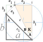
Figuren visar relationerna

	a₂	= a – a₁ = cosA·c₁ – sinA·a₃	b₁	= b + b₂ = sinA·c₁ + cosA·a₃
	a₂/c	= cos(A–B)	b₁/c	= sin(A–B)
	a₂/c	= cosA·c₁c^–1 – sinA·a₃c^–1	b₁/c	= sinA·c₁c^–1 + cosA·a₃c^–1
	a₂/c	= cosA·sinB – sinA·cosB	b₁/c	= sinA·sinB + cosA·cosB
(4)	cos(A–B)	= cosAsinB – sinAcosB	sin(A–B)	= sinAsinB + cosAcosB	(5)
		sin–B=sinB, cos–B=–cosB ;	←	projektionssymmetrierna
(1)	cos(A+B)	= cosAsinB + sinAcosB	sin(A+B)	= sinAsinB – cosAcosB	(2)

Beteckningarna (1)(2)(4)(5) refererar till ordningstalen i de totalt 14 sambanden, vidare nedan.

som tillämpade på ovanstående enhetscirkeln med r=1=r₁=r₂ med tillhörande x=sin och y=cos direkt ger komponenterna

y = y₁x₂ + x₁y₂ (1)(2) x = x₁x₂ – y₁y₂ ......... vinkelsumman

y = y₁x₂ – x₁y₂ (4)(5) x = x₁x₂ + y₁y₂ ......... vinkelskillnaden

Enhetscirkeln med r=1=r₁=r₂ medför att x/(HL)=y/(HL)=r/r₁r₂=1, (HL) respektive högerdelar.

Man har alltså ekvivalenterna totalt speciellt för sambanden i tabellen markerade (1) och (2) varur vinkelsummateoremet ges enligt

x=(x₁x₂–y₁y₂) ; y=(y₁x₂+x₁y₂) ; r=r₁r₂(=)Δ₁+Δ₂ ................ vinkelsummateoremet

summerande vinklar betyder multiplicerande hypomängder

Sambanden 3-14

Med tan=cos/sin, analogt tan=y/x, får man direkt motsvarande tangenssamband via (1)(2)

y/x =tan= (y₁x₂+x₁y₂)/(x₁x₂–y₁y₂)=(y₁x₂+x₁y₂)/[x₁x₂(1–tan₁tan₂)]=(y₁/x₁+y₂/x₂)/[1–tan₁tan₂]

=(tan₁+tan₂)/[1–tan₁tan₂]

(3) tan(A+B) = (tanA + tanB)(1 – tanAtanB)^–1

och via (4)(5) som endast har ombytta tecken

(6) tan(A–B) = (tanA – tanB)(1+ tanAtanB)^–1

Förklaring:

(7) cosAcosB = 2^–1[–sin(A+B) + sin(A–B)] ............... (2)–(5)=(7)

(8) sinAsinB = 2^–1[–sin(A+B) + sin(A–B)] ............... (2)+(5)=(8)

(9) cosAsinB = 2^–1[–cos(A+B) + cos(A–B)] ............... (1)+(4)=(9)

(10) sinAcosB = 2^–1[–cos(A+B) – cos(A–B)] ................ (1)–(4)=(10)

Med A+B=C₁ och A–B=C₂ som ger A=(C₁–C₂)/2 och B=(C₁+C₂)/2, varefter C₁ och C₂ sättes respektive A och B, ges från 7-10 sambanden 11-14.

(11) sinA–sinB = –2cos[(A+B)2^–1]cos[(A–B)2^–1]

(12) sinA+sinB = –2sin[(A+B)2^–1]sin[(A–B)2^–1]

(13) cosA+cosB = –2cos[(A+B)2^–1]sin[(A–B)2^–1]

(14) cosA–cosB = –2sin[(A+B)2^–1]cos[(A–B)2^–1]

Med reservation för eventuella skrivfel och överföringsfel.

Baskartan från 1984

Från originalarbeten i sammanställning 1984 VII,

i vidare bearbetning 2003III14 | 2012VIII16 för UNIVERSUMS HISTORIA.

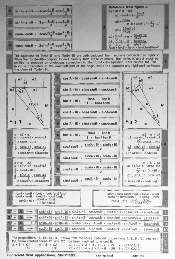
Trigonometrins tangensformer — från M2001_3.wps

TRIGONOMETRINS TANGENSFORMER från elementära samband

The tangent forms in trigonometry

THE TANGENT FORMS IN TRIGONOMETRY in PREFIXxSIN

Developing the sine function

(4) (2) (1) (3)

–sin x cos x sin x –cos x –sin x

y=sin(180–x) y=sin(90–x) y=sin x y=sin(90+x)

(1) sin x

(2) sin(90–x) = cos x

(3) sin(90+x) = –cos x

(4) sin(180±x) = –sin x

By using the elementary trigonometric connections on the given sine wave function

(1) y = sin x

we receive the other significant expressions from the given one by simply relating the y-axis in consecutive steps of 90 degrees. The figure above shows the resulting equative expressions. From these basic forms is derived the same systematic order for the corresponding derivatives. The primary form with Dn sin = –cos shows a corresponding angular displacement in 90 degrees steps according to the former order as

(1.1) Dn sin x = –cos x

(2.1) Dn cos x = sin x

(3.1) Dn –cos x = –sin x

(4.1) Dn –sin x = cos x

The tangent-forms for tangent and cotangent

(5) Dn tan = sec²

(6) Dn cot = –cosec²

If we return to the primary tables in trigonometry, number [6] in the composite forms,

tan(A–B) = (tanA – tanB)/(1+ tanAtanB)

namely re-written on the form

(1+tanAtanB)=(tanA–tanB)/tan(A–B)

we soon see the likeness with the position form itself, k = dy/dx = (y₀–y)/(x₀–x).

With

y₀ = tan x₀ and y = tan x we receive

k = d(tanx)/dx = (tanx₀ – tanx)/dx accordingly

(tanx₀ – tanx)/tandx = 1+ tanx₀tanx

Explanation:

If we recall the characteristics of the circle where the angle x is measured in radians, we see that the logical interval Δx of the angle x equals the tangent of Δx. As the aspect of Dx also is the aspect of the entire angle x, i.e., the ”line” of the arc as the radius of the circle, we arrive at the position (tanx)/∞ with the same meaning as the position x/∞, analogously

tandx = dx.

Then we receive

Dn tanx = (tanx₀ – tanx)/dx = 1+ tanx₀tanx 1+ (tanx)²

From the primary relations we know that this expression also has the equivalent

(sec x)² = 1/(sin x)². We then have found (5) that Dn tanx = (sec x)².

If we continue this investigation by inverting the tangent in number [6] in the composite forms, same as above, we find the only difference to be a negative result. We put

K = (a–b)/(1+ab) and receive

(1/a – 1/b)/(1+1/ab) = [(b–a)/ab]/[(ab+1)/ab]

= (b–a)/(1+ab) = –K

For [6] in the composite forms with its right part of the rank as reciprocal tangents it hence counts that

–tan(A–B) = (cotA–cotB)/(1+cotAcotB)

= – (tanA – tanB)/(1+ tanAtanB) ;

(cotA–cotB)/tan(A–B) = –(1+cotAcotB).

Let us thereby consider the case with the derivative to

y = cotx = 1/tanx. We put y=cotx, y₀=cotx₀ so that we get

k = dy/dx = (y₀–y)/(x₀–x)

k = d(1/tanx)/dx = d(cotx)/dx = (cotx₀ – cotx)/dx

As we see, these ranks are analog to the extract above,

(cotA – cotB)/tan(A – B) = – (1+ cotAcotB), so that we can put

(cotx₀ – cotx)/tan(x₀ – x) = – (1+ cotx₀cotx) = d(cotx)/dx. We hence have that

(cotx₀ – cotx)/tan(dx) = – (1+ cotx₀cotx). Similar to the previous order it also holds here that

tan(dx)=dx which then gives us the equivalent to the position form for cotx above according to

(cotx₀ – cotx)/dx = – (1+ cotx₀cotx) – [1+ (cotx)²]. From the primary trigonometric relations we now know that

1+ (cot)² has the equivalent 1/cos²=(cosec)². We then have found (6) that

Dn cotx = –[1+ (cotx)²] = –(cosec x)².

As we see, the orders hold tan-sec and cot-cosec so it is comparatively easy to handle and remember.

From these received connections, it is possible to reach the corresponding cyclometric tangent form expressions.

The arc functions

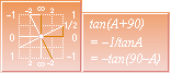
By conceiving the basic forms recently derived, rotated positively 90 degrees, a change is analogously made to the tangent forms from tanA to –1/tanA as is shown in the small illustration here on top.

By adopting the expressions to the rotation attaching the xy-axes, one receives the corresponding modified functions. As we know the tangent form to the functions sine, cosine and tangent, the tangent forms can be deduced for the corresponding arc functions by this method. The given tangent form hence is transformed through

· change of sign by positive rotation a quarter of a turn

· inverting, angular index changes from A to 90–A (see illustration above)

· (x ; y) replaces by (y ; –x)

[Normally you need some practice to immediately see the point in this description. If you don’t get it ”right ahead”, don’t despair: you are in good company; You don’t know how many times I had to walk things over, again and again and again in seemingly endless circles, before I really got to the point].

In the following workout, I will just show the simple figures with the accompanying results.

Sine function, y=sin x:

Dn y = – cosx = tanA [= y/x]

1/cosx = –1/tanA

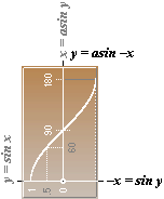
Arc Sine function, y=asin –x:

Dn y = 1/cosy = 1/√1–(siny)² = 1/√1–x²

Dn asin–x = 1/√1–x²

Dn asinx = –1/√1–x²

CoSine function, y=cos x:

Dn y = sinx = tanA [= y/x]

–1/sinx = –1/tanA

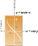
Arc CoSine function, y=acos –x:

Dn y = –1/siny = –1/√1–(cosy)² = –1/√1–x²

Dn acos–x = –1/√1–x²

Dn acosx = 1/√1–x²

Tangent function, y=tan x:

Dn y = 1/(sinx)² = tanA [= y/x]

–(sinx)² = –1/tanA

y = cot x :

Dn y = –1/(cosx)² = tanA [= y/x]

(cosx)² = –1/tanA

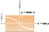
Arc Tangent function, y=atan –x:

Dn y = –(siny)² = –1/1+(tany)² = –1/1+x²

Dn atan–x = –1/1+x²

Dn atanx = 1/1+x²

y = acot–x :

Dn y = (cosy)² = 1/1+(coty)² = 1/1+x²

Dn acot–x = 1/1+x²

Dn acotx = –1/1+x²

Compilation Arc Derivatives in PREFIXxSIN:

Dn asinx = Dn acos–x = –1/√1–x²

Dn acosx = Dn asin–x = 1/√1–x²

Dn atanx = Dn acot–x = 1/1+x²

Dn acotx = Dn atan–x = –1/1+x²

VinkelkoefficientDerivatorna

The derivatives with angle coefficient

ADDING THE ANGLE COEFFICIENT

If we introduce a zooming factor or a coefficient n to the variable x, we find that the corresponding aspect ratio towards the square unit has changed. To restore the square unit in the result, we then must zoom the y-extension by the same zooming factor n. Then we directly receive from the previous developments

Dn sin nx = –n(cos nx)

Dn cos nx = n(sin nx)

Dn tan nx = n(sin nx)^–2

Dn cot nx = –n(cos nx)^–2

For the arc functions in the previous, we have respectively

[–x=sin y]_asin, [–x=cos y]_acos, [–x=tan y]_atan, [–x=cot y]_acot

where all x become squared in the end-connections, as previously shown. With a zooming factor n the end result hence relies on the square of nx for the variable with an additional n for restoring the square unit ratio. In total we hence receive for the arcs

Dn asin nx = –n/√1–(nx)²

Dn acos nx = n/√1–(nx)²

Dn atan nx = n/1+(nx)²

Dn acot nx = –n/1+(nx)²

With these details we should be fairly well prepared to meet (any of) the more sophisticated levels in related mathematics.

END.

FORMLAGARNA I HÄRLEDNING

innehåll: SÖK äMNESORD på denna sida Ctrl+F · sök ämnesord överallt i SAKREGISTER

FORMLAGARNA I HÄRLEDNING

ämnesrubriker

innehåll

FORMLAGARNA I HÄRLEDNING

Tabellen

Potensderivatan

Formlagarna

Formlagarna med utförliga härledningar

Positionsformen

Expontentiella

Trigonometriska

Arkusfunktionernas Tangensformer

Logaritmiska

APPENDIX

Vinkelsummateoremet — fullständiga 14 sambanden

Trigonometriska Baskartan från 1984

Trigonometrins tangensformer

VinkelkoefficientDerivatorna

referenser

[HOP]. HANDBOOK OF PHYSICS, E. U. Condon, McGraw-Hill 1967

Atomviktstabellen i HOP allmän referens i denna presentation, Table 2.1 s9–65—9–86.

m_n = 1,0086652u ...................... neutronmassan i atomära massenheter (u) [HOP Table 2.1 s9–65]

m_e = 0,000548598u .................. elektronmassan i atomära massenheter (u) [HOP Table 10.3 s7–155 för m_e , Table 1.4 s7–27 för u]

u = 1,66043 t27 KG .............. atomära massenheten [HOP Table 1.4 s7–27, 1967]

u = 1,66033 t27 KG .............. atomära massenheten [ENCARTA 99 Molecular Weight]

u = 1,66041 t27 KG ............... atomära massenheten [FOCUS MATERIEN 1975 s124sp1mn]

u = 1,66053886 t27 KG ........ atomära massenheten [teknisk kalkylator, lista med konstanter SHARP EL-506W (2005)]

u = 1,6605402 t27 KG .......... atomära massenheten [@INTERNET (2007) sv. Wikipedia]

u = 1,660538782 t27 KG ...... atomära massenheten [från www.sizes.com],

CODATA rekommendation från 2006 med toleransen ±0,000 000 083 t27 KG (Committe on Data for Science and Technology)]

c₀ = 2,99792458 T8 M/S ........ ljushastigheten i vakuum [ENCARTA 99 Light, Velocity, (uppmättes i början på 1970-talet)]

h = 6,62559 t34 JS ................. Plancks konstant [HOP s7–155]

e = 1,602 t19 C ...................... elektriska elementarkvantumet, elektronens laddning [FOCUS MATERIEN 1975 s666ö]

e₀ = 8,8543 t12 C/VM ............. elektriska konstanten i vakuum [FOCUS MATERIEN 1975 s666ö]

G = 6,67 t11 JM/(KG)² .......... allmänna gravitationskonstanten [FOCUS MATERIEN 1975 s666ö] — G=F(r/m)² → N(M/KG)² = NM²/(KG)² = NM·M/(KG)²=JM/(KG)²

BKL BONNERS KONVERSATIONSLEXIKON Band I-XII med Suppement A-Ö 1922-1929, Bonniers Stockholm

[BA]. BONNIERS ASTRONOMI 1978 — Det internationella standardverket om universum sammanställt vid universitetet i Cambridge

t för 10^–, T för 10⁺, förenklade exponentbeteckningar

MAC, modern akademi (Modern ACademy)

TNED

(Toroid Nuclear Electromechanical Dynamics), eller ToroidNukleära Elektromekaniska Dynamiken

är den dynamiskt ekvivalenta resultatbeskrivning som följer av härledningarna i Planckringen h=m_nc₀r_n, analogt Atomkärnans Härledning. Beskrivningen enligt TNED är relaterad, vilket innebär: alla, samtliga, detaljer gör anspråk på att vara fullständigt logiskt förklarbara och begripliga, eller så inte alls. Med TNED får därmed (således) också förstås RELATERAD FYSIK OCH MATEMATIK. Se även uppkomsten av termen TNED [Planckfraktalerna] i ATOMKÄRNANS HÄRLEDNING.

Senast uppdaterade version: 2018-12-27

*END.

Stavningskontrollerat 2012-08-20.

rester

åter till portalsidan · portalsidan är www.UniversumsHistoria.se

∫ √ τ π ħ ε UNICODE — ofta använda tecken i matematiska-tekniska-naturvetenskapliga beskrivningar

σ ρ ν ν π τ γ λ η ≠ √ ħ ω →∞ ≡

Ω Φ Ψ Σ Π Ξ Λ Θ Δ

α β γ δ ε λ θ κ π ρ τ φ σ ω ∏ √ ∑ ∂ ∆ ∫ ≤ ≈ ≥ ← ↑ → ∞ ↓

ζ ξ

Pilsymboler, direkt via tangentbordet:

Alt+24 ↑; Alt+25 ↓; Alt+26 →; Alt+27 ←; Alt+22 ▬

Alt+23 ↨ — även Alt+18 ↕; Alt+29 ↔

☺☻♥♦♣♠•◘○◙♂♀♪♫☼►◄↕‼¶§▬↨↑↓

→←∟↔▲▼ !”#$%&’()*+,

■²³¹·¨°¸÷§¶¾‗±

åter till portalsidan · portalsidan är www.UniversumsHistoria.se